
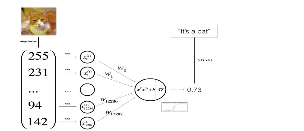
基本流程
加载数据 —> 训练模型找出 w,b —> 将 w,b 代入预测函数 —> 预测
实现
数据加载
数据是给好的hd5文件低像素图片
导入库 —> 加载数据集 —> 数据重塑
import numpy as np  # 导入NumPy库,用于科学计算
import h5py  # 导入h5py库,用于处理HDF5文件

def load_dataset():
    # 打开训练数据集文件,以只读模式读取
    train_dataset = h5py.File('datasets/train_catvnoncat.h5', "r")
    # 从训练数据集中提取特征数据,并转换为NumPy数组
    train_set_x_orig = np.array(train_dataset["train_set_x"][:])
    # 从训练数据集中提取标签数据,并转换为NumPy数组
    train_set_y_orig = np.array(train_dataset["train_set_y"][:])

    # 打开测试数据集文件,以只读模式读取
    test_dataset = h5py.File('datasets/test_catvnoncat.h5', "r")
    # 从测试数据集中提取特征数据,并转换为NumPy数组
    test_set_x_orig = np.array(test_dataset["test_set_x"][:])
    # 从测试数据集中提取标签数据,并转换为NumPy数组
    test_set_y_orig = np.array(test_dataset["test_set_y"][:])

    # 从测试数据集中提取类别信息,并转换为NumPy数组
    classes = np.array(test_dataset["list_classes"][:])

    # 将训练标签数据重塑为二维数组,形状为(1, 样本数量)
    train_set_y_orig = train_set_y_orig.reshape((1, train_set_y_orig.shape[0]))
    # 将测试标签数据重塑为二维数组,形状为(1, 样本数量)
    test_set_y_orig = test_set_y_orig.reshape((1, test_set_y_orig.shape[0]))

    # 返回训练和测试数据集的特征、标签以及类别信息
    return train_set_x_orig, train_set_y_orig, test_set_x_orig, test_set_y_orig, classes
我们可以模拟一个简单的 HDF5 数据集结构,并使用它来测试数据加载和处理功能
import numpy as np

h5demo = {
    "list_classes": [0, 1],  # 类别标签
    "train_set_x": [
        [1, 2, 3, 4, 5],
        [1, 2, 3, 4, 5],
        [1, 2, 3, 4, 5],
        [1, 2, 3, 4, 5],
        [1, 2, 3, 4, 5]
    ],
    "train_set_y": [0, 1, 0, 1, 0],  # 训练集标签
    "test_set_x": [
        [5, 4, 3, 2, 1],
        [5, 4, 3, 2, 1],
        [5, 4, 3, 2, 1],
        [5, 4, 3, 2, 1],
        [5, 4, 3, 2, 1]
    ],
    "test_set_y": [1, 0, 1, 0, 1]  # 测试集标签
}


print(h5demo["list_classes"])
print(h5demo["list_classes"][:])
print(np.array(h5demo["train_set_x"][:]))
[0, 1]
[0, 1]
[[1 2 3 4 5]
[1 2 3 4 5]
[1 2 3 4 5]
[1 2 3 4 5]
[1 2 3 4 5]]现在打印 train_set_x_orig 和 train_set_y_orig 的形状,观察数据的结构
# 加载数据集
train_set_x_orig, train_set_y_orig, test_set_x_orig, test_set_y_orig, classes = load_dataset()

# 打印训练集特征数据的形状
print("train_set_x_orig shape:", train_set_x_orig.shape)

# 打印训练集标签数据的形状
print("train_set_y_orig shape:", train_set_y_orig.shape)
train_set_x_orig shape: (209, 64, 64, 3)
train_set_y_orig shape: (1, 209)-
train_set_x_orig shape: (209, 64, 64, 3): 这表示训练集特征数据的形状。具体来说:
-
209 是样本数量,表示有 209 张图片。
-
64 是图片的高度和宽度,表示每张图片是 64x64 像素的正方形。
-
3 是通道数,表示每张图片是彩色的(RGB)。
-
-
train_set_y_orig shape: (1, 209): 这表示训练集标签数据的形状。具体来说:
-
1 是标签的维度,表示每个样本只有一个标签。
-
209 是样本数量,表示每个样本对应一个标签。
-
解释一下维度
-
标量: 没有维度,因为它是一个单一的数值。a=1
-
向量: 只有一个维度,表示为一个列或行。a=[1,2,3]
-
矩阵: 有两个维度,表示为行和列。a=[[1,2,3],[1,2,3]]
-
张量: 有三个或更多维度,可以看作是多个矩阵的集合。a=[[[1]],[[2]],[[3]]]
scalar = np.array(1)  # 标量,0维
vector = np.array([1, 2, 3])  # 向量,1维
matrix = np.array([[1, 2, 3],[1,2,3]])  # 矩阵,2维
tensor = np.array([[[1], [2]], [[3], [4]]])  # 张量,3维

# 打印每个数组的维数
print("Scalar ndim:", scalar.ndim)  # 输出: 0
print("Vector ndim:", vector.ndim)  # 输出: 1
print("Matrix ndim:", matrix.ndim)  # 输出: 2
print("Tensor ndim:", tensor.ndim)  # 输出: 3
解释一下重塑
- 原始的 test_set_y_orig 可能是一维数组,形状为 (样本数量,)。将其重塑为(1,样本数量)使得后续的矩阵运算更加方便和一致,尤其是在与其他二维数组(如特征矩阵)进行运算时。 (1, 样本数量) 表示一个行向量,其中有 样本数量 个元素。
import numpy as np

h5demo = {
    "train_set_y": [0, 1, 0, 1, 0]# 训练集标签
}

train_set_y = np.array(h5demo["train_set_y"][:]) #转化nump数组

print("转换前: ")
print(train_set_y)
print(train_set_y.shape)
print(train_set_y.ndim)

print("\n换后: ")
train_set_y = train_set_y.reshape((1,train_set_y.shape[0]))
print(train_set_y)
print(train_set_y.shape)
print(train_set_y.ndim)
转换前:
[0 1 0 1 0]
(5,)
1
换后:
[[0 1 0 1 0]]
(1, 5)
2数据处理
m_train = train_set_x_orig.shape[0]
m_test = test_set_x_orig.shape[0]
num_px = test_set_x_orig.shape[1] # 由于我们的图片是正方形的,所以长宽相等

train_set_x_flatten = train_set_x_orig.reshape(train_set_x_orig.shape[0], -1).T
test_set_x_flatten = test_set_x_orig.reshape(test_set_x_orig.shape[0], -1).T

train_set_x = train_set_x_flatten/255.
test_set_x = test_set_x_flatten/255.
数据展平
操作
-
reshape(train_set_x_orig.shape[0], -1) 将每张图片展平成一个一维向量。
-
-1 表示自动计算展平后的维度。对于一张 64x64 的彩色图片,展平后会变成一个长度为 12288 的向量(64 * 64 * 3)。
-
.T 是转置操作,将数据从 (样本数量, 特征数) 转换为 (特征数, 样本数量),这在机器学习中是一个常见的格式。
为什么
-
展平操作将每张图片的像素值展平为一个一维向量,使得每个样本都可以用一个向量表示。
-
这种格式便于输入到机器学习模型中进行训练。
数据标准化
操作
-
将展平后的数据除以 255,将像素值缩放到 [0, 1] 的范围内。
-
这一步是为了加速模型的训练过程,并提高模型的稳定性。为什么标准化:
为什么
-
标准化可以使特征具有相同的尺度,避免某些特征对模型的影响过大。
-
通过缩放到 [0, 1],可以加速梯度下降的收敛。
模型初始化
对于线性模型,我们通常需要初始化权重和偏置。
def initialize_with_zeros(dim):
    # 初始化权重向量w为零向量,形状为(dim, 1)
    w = np.zeros((dim, 1))
    # 初始化偏置b为0
    b = 0
    # 返回初始化的权重和偏置
    return w, b
import numpy as np
demo = np.zeros((2,3))
print(demo)
demo1 = np.zeros((2,1))
print(demo1)
'''
[[0. 0. 0.]
[0. 0. 0.]]
[[0.]
[0.]]
'''前向传播和反向传播
def propagate(w, b, X, Y):
    # 获取样本数量
    m = X.shape[1]

    # 前向传播:计算激活值A
    A = sigmoid(np.dot(w.T, X) + b)
    # 计算损失函数的值,使用交叉熵损失
    cost = -np.sum(Y * np.log(A) + (1 - Y) * np.log(1 - A)) / m

    # 反向传播:计算梯度
    dZ = A - Y
    dw = np.dot(X, dZ.T) / m
    db = np.sum(dZ) / m

    # 将梯度存储在字典中
    grads = {
        "dw": dw,
        "db": db
    }

    # 返回梯度和损失
    return grads, cost
这里前向传播和反向传播直接带的公示,现在简要讲解一下原理
前向传播是指将输入数据通过神经网络传递,计算输出的过程。其主要目的是计算模型的预测值。
-
输入层:
- 输入数据 XX 被传递到网络的第一层。
-
隐藏层(如果有):
-
每个神经元接收输入,计算加权和,并通过激活函数得到输出。
-
公式:a[l]=σ(W[l]a[l−1]+b[l])a[l]=σ(W[l]a[l−1]+b[l])
-
其中,W[l]W[l] 是权重矩阵,b[l]b[l] 是偏置,σσ 是激活函数。
-
-
输出层:
- 最后一层的输出即为模型的预测值 Y^Y^。
-
损失计算:
- 计算预测值与真实值之间的差异,通常使用损失函数(如均方误差、交叉熵等)。
反向传播是指通过计算损失函数的梯度,更新模型参数的过程。其主要目的是最小化损失函数。
-
损失函数的梯度:
- 计算损失函数对输出层的梯度。
-
链式法则:
- 使用链式法则计算每一层的梯度。
-
参数更新:
- 使用梯度下降法更新权重和偏置。
简单来说,前向传播就是输入数据,计算损失;反向传播就是根据损失,调整参数。
模型优化
def optimize(w, b, X, Y, num_iterations, learning_rate, print_cost=False):
    costs = []  # 用于存储每100次迭代的损失值

    for i in range(num_iterations):
        # 计算梯度和损失
        grads, cost = propagate(w, b, X, Y)

        # 从字典中提取梯度
        dw = grads["dw"]
        db = grads["db"]

        # 更新权重和偏置
        w = w - learning_rate * dw
        b = b - learning_rate * db

        # 每100次迭代记录一次损失
        if i % 100 == 0:
            costs.append(cost)
            if print_cost:
                print("迭代的次数: %i, 误差值: %f" % (i, cost))

    # 返回优化后的参数和损失
    params = {
        "w": w,
        "b": b
    }

    return params, costs
模型预测函数
def predict(w, b, X):
    m = X.shape[1]  # 样本数量
    Y_prediction = np.zeros((1, m))  # 初始化预测结果为零
    A = sigmoid(np.dot(w.T, X) + b)  # 计算激活值

    for i in range(A.shape[1]):
        # 如果激活值大于0.5,预测为1,否则为0
        if A[0, i] > 0.5:
            Y_prediction[0, i] = 1
        else:
            Y_prediction[0, i] = 0

    return Y_prediction
构建和训练模型
我们将使用一个函数来整合所有步骤,包括初始化参数、优化参数、预测结果,并评估模型的性能。
def model(X_train, Y_train, X_test, Y_test, num_iterations=2000, learning_rate=0.5, print_cost=False):
    '''
        train_set_x 和 train_set_y: 训练集的特征和标签。
        test_set_x 和 test_set_y: 测试集的特征和标签。
        num_iterations: 迭代次数,决定了优化过程的持续时间。
        learning_rate: 学习率,控制每次更新的步长。
        print_cost: 是否打印每 100 次迭代的损失值。

    '''


    # 初始化参数
    w, b = initialize_with_zeros(X_train.shape[0])

    # 优化参数
    params, costs = optimize(w, b, X_train, Y_train, num_iterations, learning_rate, print_cost)

    # 从优化结果中提取参数
    w = params["w"]
    b = params["b"]

    # 预测训练集和测试集的结果
    Y_prediction_test = predict(w, b, X_test)
    Y_prediction_train = predict(w, b, X_train)

    # 打印训练集和测试集的准确率
    print("训练集准确率: {} %".format(100 - np.mean(np.abs(Y_prediction_train - Y_train)) * 100))
    print("测试集准确率: {} %".format(100 - np.mean(np.abs(Y_prediction_test - Y_test)) * 100))

    # 返回模型信息
    d = {
        "costs": costs,
        "Y_prediction_test": Y_prediction_test,
        "Y_prediction_train": Y_prediction_train,
        "w": w,
        "b": b,
        "learning_rate": learning_rate,
        "num_iterations": num_iterations
    }
    return d
运行模型
运行之前,看一下数据集中的图片怎么样
index = 30
plt.imshow(train_set_x_orig[index])
print ("标签为" + str(train_set_y[:, index]) + ", 这是一个'" + classes[np.squeeze(train_set_y[:, index])].decode("utf-8") +  "' 图片.")
plt.show()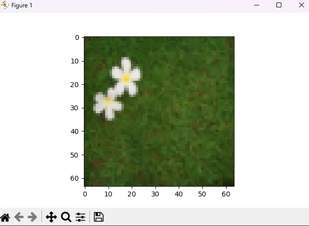
标签为[0], 这是一个'non-cat' 图片.也是能够正常展示
# 运行模型
d = model(train_set_x, train_set_y, test_set_x, test_set_y, num_iterations=2000, learning_rate=0.005, print_cost=True)
==》
迭代的次数: 0, 误差值: 0.693147
迭代的次数: 100, 误差值: 0.584508
迭代的次数: 200, 误差值: 0.466949
迭代的次数: 300, 误差值: 0.376007
迭代的次数: 400, 误差值: 0.331463
迭代的次数: 500, 误差值: 0.303273
迭代的次数: 600, 误差值: 0.279880
迭代的次数: 700, 误差值: 0.260042
迭代的次数: 800, 误差值: 0.242941
迭代的次数: 900, 误差值: 0.228004
迭代的次数: 1000, 误差值: 0.214820
迭代的次数: 1100, 误差值: 0.203078
迭代的次数: 1200, 误差值: 0.192544
迭代的次数: 1300, 误差值: 0.183033
迭代的次数: 1400, 误差值: 0.174399
迭代的次数: 1500, 误差值: 0.166521
迭代的次数: 1600, 误差值: 0.159305
迭代的次数: 1700, 误差值: 0.152667
迭代的次数: 1800, 误差值: 0.146542
迭代的次数: 1900, 误差值: 0.140872
训练集准确率: 99.04306220095694 %
测试集准确率: 70.0 %
我可以打印出成本的变化情况,即每次调整参数实际值与预测值的误差,应该是下降的。
# 从字典 d 中提取成本列表,并去除不必要的维度,就是把二维的转成一维的,便于绘图
costs = np.squeeze(d['costs'])

# 使用 Matplotlib 绘制成本随迭代次数变化的折线图
plt.plot(costs)

# 设置 y 轴标签为 'cost',表示图中每个点的 y 值代表损失函数的值
plt.ylabel('cost')  # 成本

# 设置 x 轴标签为 'iterations (per hundreds)',表示图中每个点的 x 值代表迭代次数,以 100 为单位
plt.xlabel('iterations (per hundreds)')  # 横坐标为训练次数,以100为单位

# 设置图表的标题,显示当前使用的学习率
plt.title("Learning rate =" + str(d["learning_rate"]))

# 显示绘制的图表
plt.show()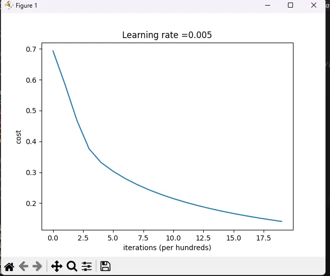
接着,我们可以看看基于损失函数,学习率对模型造成的影响。(一个好的学习率,能使结果更加准确)
learning_rates = [0.01, 0.001, 0.0001]
models = {}
for i in learning_rates:
    print ("学习率为: " + str(i) + "时")
    models[str(i)] = model(train_set_x, train_set_y, test_set_x, test_set_y, num_iterations = 1500, learning_rate = i, print_cost = False)
    print ('\n' + "-------------------------------------------------------" + '\n')

for i in learning_rates:
    plt.plot(np.squeeze(models[str(i)]["costs"]), label= str(models[str(i)]["learning_rate"]))

plt.ylabel('cost')
plt.xlabel('iterations (hundreds)')

legend = plt.legend(loc='upper center', shadow=True)
frame = legend.get_frame()
frame.set_facecolor('0.90')
plt.show()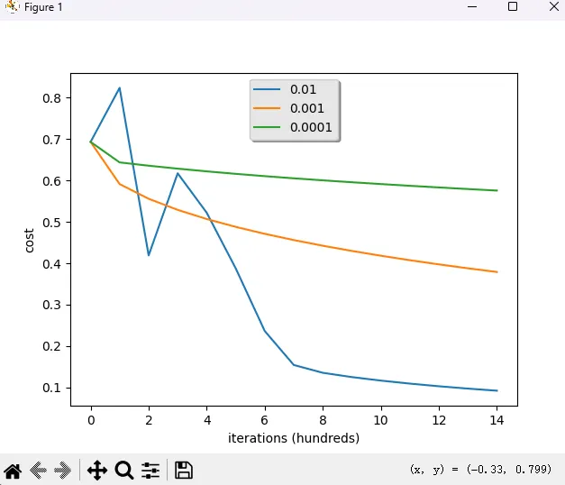
学习率为: 0.01时
训练集准确率: 99.52153110047847 %
测试集准确率: 68.0 %

-------------------------------------------------------

学习率为: 0.001时
训练集准确率: 88.99521531100478 %
测试集准确率: 64.0 %

-------------------------------------------------------

学习率为: 0.0001时
训练集准确率: 68.42105263157895 %
测试集准确率: 36.0 %

-------------------------------------------------------
这里选定学习率为 0.01
测试
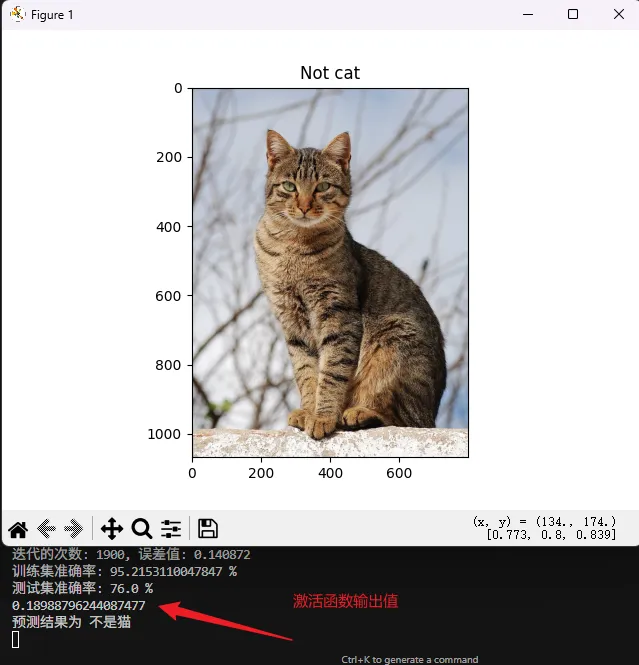
通过模型训练我们找到了合适的 w,b,下一步就只需要拿这个 w,b 带入预测函数去测试图片了。

# 读取图像文件并将其转换为 NumPy 数组
image = np.array(plt.imread(fname))

# 调整图像大小为 (num_px, num_px),并展平为一维向量
# 使用 skimage.transform 的 resize 函数,mode='reflect' 用于处理边界
my_image = tf.resize(image, (num_px, num_px), mode='reflect').reshape((1, num_px*num_px*3)).T

# 使用训练好的模型预测图像的类别,返回 0 或 1
my_predicted_image = predict(d["w"], d["b"], my_image)   # 返回 0 或 1

# 判断预测结果并输出相应的文本和设置图像标题
if int(np.squeeze(my_predicted_image)) == 0:
    print("预测结果为 不是猫")  # 如果预测结果为 0,输出“不是猫”
    plt.title("Not cat")  # 设置图像标题为“不是猫”
else:
    print("预测结果为 猫")  # 如果预测结果为 1,输出“猫”
    plt.title("Is cat")  # 设置图像标题为“猫”

# 显示图像
plt.imshow(image)
plt.show()
但是对真实图片来说,效果真的很差,可能因为数据集是像素图像,训练次数不够,并且这是一个单神经元网络。
没办法,最后再测一下测试数据里的内容。
# 选择测试集中的一个图像索引
index = 0  # 你可以更改这个索引以选择不同的图像
# 提取图像数据
single_test_image = test_set_x[:, index].reshape((num_px, num_px, 3))
# 进行预测
single_test_image_flatten = test_set_x[:, index].reshape((num_px*num_px*3, 1))
predicted_label = predict(d["w"], d["b"], single_test_image_flatten)
# 显示图像
plt.imshow(single_test_image)
plt.title("Is cat" if int(np.squeeze(predicted_label)) == 1 else "Not cat")
plt.show()
# 输出预测结果
print("这张图的标签是 " + str(test_set_y[0, index]) + ", 预测结果是 " + ("猫" if int(np.squeeze(predicted_label)) == 1 else "不是猫"))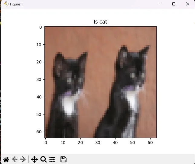
代码
import numpy as np
import matplotlib.pyplot as plt
import h5py
import skimage.transform as tf

def load_dataset():
    train_dataset = h5py.File('datasets/train_catvnoncat.h5', "r") # 加载训练数据
    train_set_x_orig = np.array(train_dataset["train_set_x"][:]) # 从训练数据中提取出图片的特征数据
    train_set_y_orig = np.array(train_dataset["train_set_y"][:]) # 从训练数据中提取出图片的标签数据

    test_dataset = h5py.File('datasets/test_catvnoncat.h5', "r") # 加载测试数据
    test_set_x_orig = np.array(test_dataset["test_set_x"][:])
    test_set_y_orig = np.array(test_dataset["test_set_y"][:])

    classes = np.array(test_dataset["list_classes"][:]) # 加载标签类别数据,这里的类别只有两种,1代表有猫,0代表无猫

    train_set_y_orig = train_set_y_orig.reshape((1, train_set_y_orig.shape[0])) # 把数组的维度从(209,)变成(1, 209),这样好方便后面进行计算
    test_set_y_orig = test_set_y_orig.reshape((1, test_set_y_orig.shape[0])) # 从(50,)变成(1, 50)

    return train_set_x_orig, train_set_y_orig, test_set_x_orig, test_set_y_orig, classes

train_set_x_orig, train_set_y, test_set_x_orig, test_set_y, classes = load_dataset()

# # 我们要清楚变量的维度,否则后面会出很多问题。下面我把他们的维度打印出来。
# print ("train_set_x_orig shape: " + str(train_set_x_orig.shape))
# print ("train_set_y shape: " + str(train_set_y.shape))
# print ("test_set_x_orig shape: " + str(test_set_x_orig.shape))
# print ("test_set_y shape: " + str(test_set_y.shape))

m_train = train_set_x_orig.shape[0]
m_test = test_set_x_orig.shape[0]
num_px = test_set_x_orig.shape[1] # 由于我们的图片是正方形的,所以长宽相等

# print ("训练样本数: m_train = " + str(m_train))
# print ("测试样本数: m_test = " + str(m_test))
# print ("每张图片的宽/高: num_px = " + str(num_px))

train_set_x_flatten = train_set_x_orig.reshape(train_set_x_orig.shape[0], -1).T
test_set_x_flatten = test_set_x_orig.reshape(test_set_x_orig.shape[0], -1).T


# 下面我们对特征数据进行了简单的标准化处理(除以255,使所有值都在[0,1]范围内)
# 为什么要对数据进行标准化处理呢?简单来说就是为了方便后面进行计算,详情以后再给大家解释

train_set_x = train_set_x_flatten/255.
test_set_x = test_set_x_flatten/255.


def sigmoid(z):
    s  = 1 / (1 + np.exp(-z))
    return s


def initialize_with_zeros(dim):

    w = np.zeros((dim,1))
    b = 0

    return w, b

def propagate(w, b, X, Y):

    m = X.shape[1]

    A = sigmoid(np.dot(w.T, X) + b)
    cost = -np.sum(Y*np.log(A) + (1-Y)*np.log(1-A)) / m

    dZ = A - Y
    dw = np.dot(X, dZ.T) / m
    db = np.sum(dZ) /m

    grads = {
        "dw":dw,
        "db":db
    }

    return grads, cost

def optimize(w, b, X, Y, num_iterations, learning_rate, print_cost = False):
    costs = []

    for i in range(num_iterations):
        grads, cost = propagate(w, b, X, Y)

        dw = grads["dw"]
        db = grads["db"]

        w = w - learning_rate * dw
        b = b - learning_rate * db

        if i % 100 == 0:
            costs.append(cost)
            if print_cost:
                print ("迭代的次数: %i, 误差值: %f" % (i,cost))

    params = {
        "w":w,
        "b":b
    }

    return params, costs

def predict(w, b, X):
    m = X.shape[1]  # 样本数量
    Y_prediction = np.zeros((1, m))  # 初始化预测结果为零
    A = sigmoid(np.dot(w.T, X) + b)  # 计算激活值

    for i in range(A.shape[1]):
        # 如果激活值大于0.5,预测为1,否则为0
        if A[0, i] > 0.5:
            Y_prediction[0, i] = 1
        else:
            Y_prediction[0, i] = 0

    return Y_prediction

def model(X_train, Y_train, X_test, Y_test, num_iterations = 2000, learning_rate = 0.5, print_cost = False):
    w, b = initialize_with_zeros(X_train.shape[0])

    params, costs = optimize(w, b, X_train, Y_train, num_iterations, learning_rate, print_cost)

    w = params["w"]
    b = params["b"]

    Y_prediction_test = predict(w, b, X_test)
    Y_prediction_train = predict(w, b, X_train)

    print("训练集准确率: {} %".format(100 - np.mean(np.abs(Y_prediction_train - Y_train)) * 100))
    print("测试集准确率: {} %".format(100 - np.mean(np.abs(Y_prediction_test - Y_test)) * 100))

    d = {
        "costs":costs,
        "Y_prediction_test":Y_prediction_test,
        "Y_prediction_train":Y_prediction_train,
        "w":w,
        "b":b,
        "learning_rate":learning_rate,
        "num_iterations":num_iterations
    }
    return d


d = model(train_set_x, train_set_y, test_set_x, test_set_y, num_iterations = 2000, learning_rate = 0.005, print_cost = True)


# index = 11
# plt.imshow(train_set_x_orig[index])
# print ("标签为" + str(train_set_y[:, index]) + ", 这是一个'" + classes[np.squeeze(train_set_y[:, index])].decode("utf-8") +  "' 图片.")
# plt.show()


# costs = np.squeeze(d['costs'])
# plt.plot(costs)
# plt.ylabel('cost') # 成本
# plt.xlabel('iterations (per hundreds)') # 横坐标为训练次数,以100为单位
# plt.title("Learning rate =" + str(d["learning_rate"]))
# plt.show()

# learning_rates = [0.01, 0.001, 0.0001]
# models = {}
# for i in learning_rates:
#     print ("学习率为: " + str(i) + "时")
#     models[str(i)] = model(train_set_x, train_set_y, test_set_x, test_set_y, num_iterations = 1500, learning_rate = i, print_cost = False)
#     print ('\n' + "-------------------------------------------------------" + '\n')

# for i in learning_rates:
#     plt.plot(np.squeeze(models[str(i)]["costs"]), label= str(models[str(i)]["learning_rate"]))

# plt.ylabel('cost')
# plt.xlabel('iterations (hundreds)')

# legend = plt.legend(loc='upper center', shadow=True)
# frame = legend.get_frame()
# frame.set_facecolor('0.90')
# plt.show()


# my_image = "cat1.png"
# fname = "image/" + my_image
# image = np.array(plt.imread(fname))
# my_image = tf.resize(image,(num_px,num_px), mode='reflect').reshape((1, num_px*num_px*3)).T
# my_predicted_image = predict(d["w"], d["b"], my_image)   # 返回 0 或 1

# print(my_predicted_image)
# if int(np.squeeze(my_predicted_image)) == 0:
#     print("预测结果为 不是猫")
#     plt.title("Not cat")
# else:
#     print("预测结果为 猫")
#     plt.title("Is cat")

# plt.imshow(image)
# plt.show()


# 选择测试集中的一个图像索引
index = 0  # 你可以更改这个索引以选择不同的图像
# 提取图像数据
single_test_image = test_set_x[:, index].reshape((num_px, num_px, 3))
# 进行预测
single_test_image_flatten = test_set_x[:, index].reshape((num_px*num_px*3, 1))
predicted_label = predict(d["w"], d["b"], single_test_image_flatten)
# 显示图像
plt.imshow(single_test_image)
plt.title("Is cat" if int(np.squeeze(predicted_label)) == 1 else "Not cat")
plt.show()
# 输出预测结果
print("这张图的标签是 " + str(test_set_y[0, index]) + ", 预测结果是 " + ("猫" if int(np.squeeze(predicted_label)) == 1 else "不是猫"))


'''
流程

加载数据 --> 训练模型找出 w,b  --> 将 w,b 代入预测函数 --> 预测
'''
像素数据在库里。
后记
感受了一波半自动写模型,无奈菜的没边,各种问题最后都会铺面而来。
对于数据集的处理,模型逻辑代码,测试功能的编写都有待欠缺。等着下一次优化,一定能准确识别猫猫。
为了不让自己太过难堪,决定先去 py 一下别人的猫识别程序,不过他们的可能就不仅仅是猫识别了,QAQ。